The power of graphs for risk forecast
Overview
Risk Analysis consists in checking the critical points that may present non-conformity during the execution of a particular project or activity.
Financial risk analysis consists of assessing the uncertainties related to a company’s financial operations, which include from cash flow management to the allocation of resources to investments.
The purpose of the financial risk analysis is to assist in the decision making by the company manager to avoid undesirable risks or create plans to minimize their impact on the company’s accounts.
Our study proposes the use of a graph-based data model to assess and manage the financial risk of a bank’s clients. We used Neo4j 3.3.1 as our Graph Database solution for this entire study.
Data
To achieve our requirements regarding risk analysis, firstly we designed the data model that contains all the information we need for risk forecasting. Our data model is shown in Figure 1.
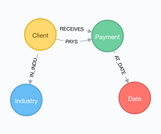
This model is at the same time simple enough and semantically complete. It allows representing the information about a Client and its Industry and also maps each Payment made at a certain Date.
Each node has the following attributes:
Client{
   id Integer;
   name String;
}

Industry{
   id Integer;
   name String;
}

Payment{
   id Integer;
   value Float;
}

Date{
   date String;
}
These nodes are related by a set of different relationships. A Client can be related to a Payment through two different Relationships: PAYS or RECEIVES. A Payment must be linked to a Date by the relationship AT_DATE. Finally, each Client belongs to one or more Industry, and it can be represented using the relationship IN_INDUSTRY.
Managing Risk Using Graphs
Having our graph model populated with our test data, we can start implementing search algorithms to evaluate the impact of each client in a certain Client-Payment chain. To be able to prove our model and use case, we populated our graph with 100 clients in 5 different industries and generated 1000 payments between them.
The first step to risk analysis is to identify our root node, the client that will be used as the point of interest in our study.
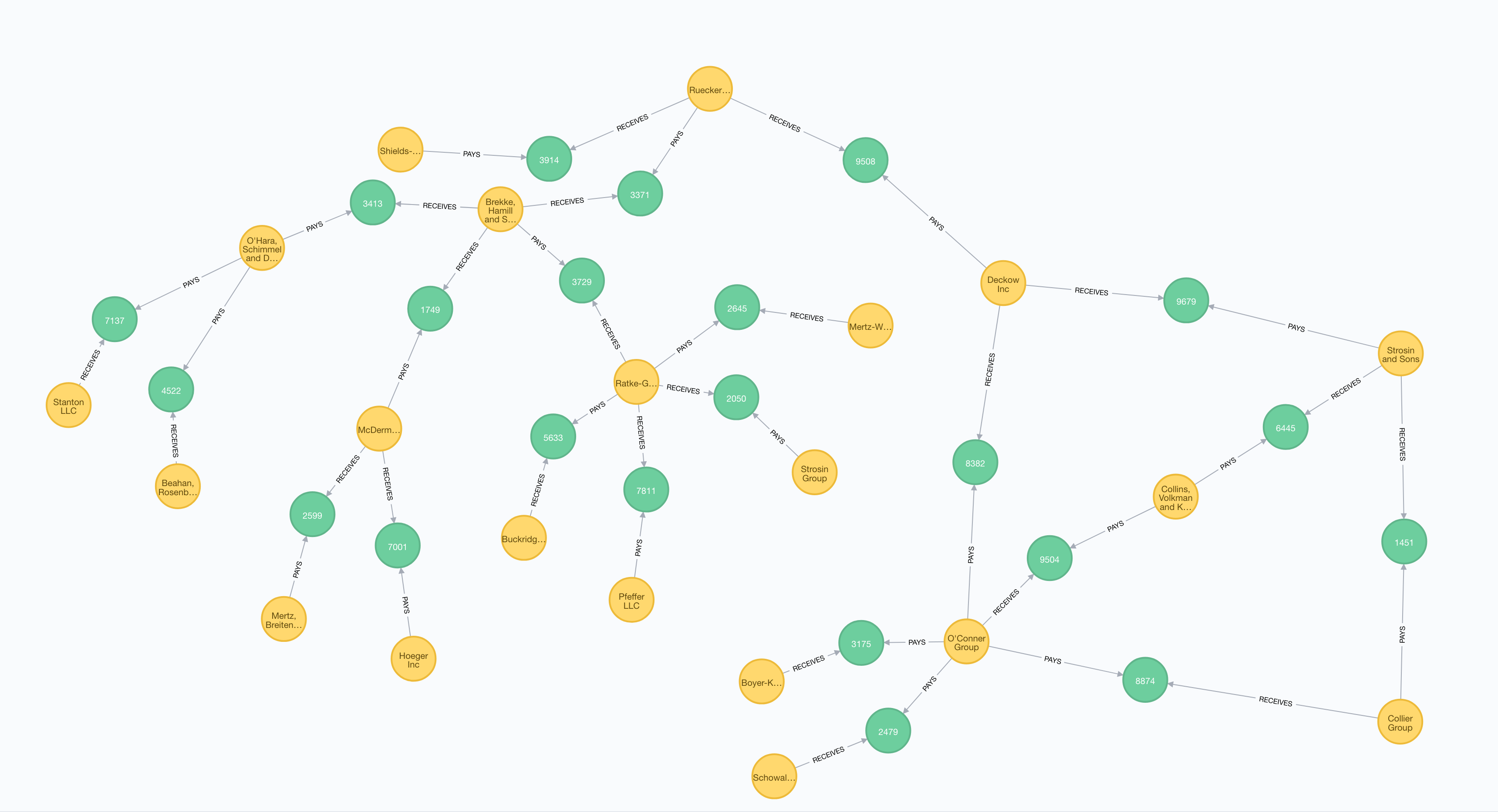
For test proposes, we had chosen the fictional Client named Ruecker-Bartoletti to be our root node. Having our root identified, we need to define the depth of our risk chain, in this case, we will handle three Client levels from the root node.
The cypher statement bellow is used to show us our payment chain (cash flow management) of depth 3, starting from our root node.
MATCH (root:Client{id:25})
CALL apoc.path.expand(root,"PAYS|RECEIVES",">Client|Payment",1,6) YIELD path
RETURN *
The example above uses the Awesome Procedures On Cypher (APOC) plugin. This Neo4j plugin allows a fast use of different graph algorithms. In the example, we used the method expand, that receives a start point (root), a list of possible relationships (PAYS and RECEIVES), the node label that we want in this expand task (Client and Payment) and, the minimum and maximum depth (1 to 6). Note that we use 6 instead of 3 because it considers the intermediate nodes: Payment.
Of course, that just displaying our chain is not enough for our risk analysis study. To identify the risk impact of each client in this chain we have to traverse the graph and assess each Payment and Client, to measure its influence, both local (on its own subtree: Parent and Children nodes) and global (its impact on the entire tree or, in other words, its impact on the root node).
The Cypher statement below shows all the steps, from identifying the root node until evaluating global and local impact.
// STEP 1
MATCH (r:Client{id:25})--(p:Payment)
WITH r,sum(p.value) as tr

// STEP 2
MATCH (r)--(p:Payment)--(l1:Client)
WITH r,tr
,l1,sum(p.value) as val1

// STEP 3
MATCH (l1)--(p:Payment)
WITH r,tr
,l1,val1
,sum(p.value)-val1 as t1

// STEP 4
OPTIONAL MATCH (l1)--(p:Payment)--(l2:Client)
WHERE NOT l2=r
WITH r,tr
,l1,val1,t1
,l2,sum(p.value) as val2

// STEP 5
OPTIONAL MATCH (l2)--(p:Payment)
WITH r,tr
,t1,l1,val1
,l2,val2
,sum(p.value)-val2 as t2

// STEP 6
OPTIONAL MATCH (l2)--(p:Payment)--(l3:Client)
WHERE NOT l3=r AND NOT l3=l1
WITH r,tr
,l1,t1,val1
,l2,t2,val2
,l3,sum(p.value) as val3


// STEP 7
WITH
r.name as r,tr,
CASE WHEN tr = 0
THEN 0
ELSE val1/tr END AS p1
,l1.name as l1,
CASE WHEN t1 = 0
THEN 0
ELSE val2/t1 END AS p2
,l2.name as l2,
CASE WHEN t2 = 0
THEN 0
ELSE val3/t2 END AS p3
,l3.name as l3

// STEP 8
WITH
r,tr,l1,p1
,p3,l3,
CASE WHEN p1=0 OR l2 IS  NULL
THEN p1
ELSE p2*p1 END AS  p2Final
,p2,l2

// STEP 9
WITH
r,tr,l1,p1
,p2,l2,p2Final,
CASE WHEN p2=0 OR l3 IS NULL
THEN p2Final
ELSE p3*p2Final END AS  p3Final
,p3,l3


// STEP 10
RETURN r as RootNode
,p1 as Local_Impact_1, p1 as Overall_Impact_1,l1 as Level1_Node
,p2 as Local_Impact_2, p2Final as Overall_Impact_2, l2 as L2vel2_Node
,p3 as Local_Impact_3, p3Final as Overall_Impact_3, l3 as Level3_Node
ORDER BY r,l1,l2,l3
The example above can be split into 10 steps:
- Step 1 - Locate the root node and the total amount of its payments (paid and received);
- Step 2 - Start evaluating the first level of our tree. We also sum all payments for every client at this level;
- Step 3 - To be able to continue expanding the tree, in this step we need to find the “local roots” and the total amount of their payments;
- Step 4 - Same as Step 2, but for level 2;
- Step 5 - Same as Step 3, but this time, we need to find the roots at level 2;
- Step 6 - Same as Step 2, but for level 3;
- Step 7 - At this step, we start evaluating the risk impact at each level (or sub-tree). We assess the impact of the payments to/from a child node for its Parent (root);
- Steps 8 and 9 - As our level 1 is already both global and local in terms of impact (this level is directed linked with the root), we start on level 2. At these step, we assess the global impact o each node in the entire tree (direct impact to our root node);
- Step 10 - Here, we return the data.
In our study, we expanded our tree until level 3, but it could grow how many levels we want. Following our Cypher statement above, we could easily adapt steps 3 and 4 for other levels, as we did in steps 5 and 6 for level 3. Also, we need to replicate Step 8 (as we did in step 9) for the remaining levels we want.
Table 1 shows the results regarding the local impact of each Client node.
| Root | Local Impact L1 | Level 1 Node | Local Impact L2 | Level 2 Node | Local Impact L3 | Level 3 Node |
|---|---|---|---|---|---|---|
| Ruecker-Bartoletti | 0.200738403 | Brekke, Hamill and Schroeder | 0.19671578 | McDermott-Kihn | 0.729270833 | Hoeger Inc |
| 0.270729167 | Mertz, Breitenberg and Kuhn | |||||
| 0.383871331 | O'Hara, Schimmel and Douglas | 0.387854876 | Beahan, Rosenbaum and Zboncak | |||
| 0.612145124 | Stanton LLC | |||||
| 0.419412889 | Ratke-Gutmann | 0.310546337 | Buckridge-Armstrong | |||
| 0.145818402 | Mertz-Weissnat | |||||
| 0.430619108 | Pfeffer LLC | |||||
| 0.113016153 | Strosin Group | |||||
| 0.566188293 | Deckow Inc | 0.464093904 | O'Conner Group | 0.132115513 | Boyer-Kohler | |
| 0.369257656 | Collier Group | |||||
| 0.395472703 | Collins, Volkman and Kunze | |||||
| 0.103154128 | Schowalter and Sons | |||||
| 0.535906096 | Strosin and Sons | 0.183763931 | Collier Group | |||
| 0.816236069 | Collins, Volkman and Kunze | |||||
| 0.233073304 | Shields-Hyatt |
Similar to the previous table, Table 2 shows the global impact for the tree nodes.
| Root | Overall Impact L1 | Level 1 Node | Overall Impact L2 | Level 2 Node | Overall Impact L3 | Level 3 Node |
|---|---|---|---|---|---|---|
| Ruecker-Bartoletti | 0.200738403 | Brekke, Hamill and Schroeder | 0.039488412 | McDermott-Kihn | 0.028797747 | Hoeger Inc |
| 0.010690665 | Mertz, Breitenberg and Kuhn | |||||
| 0.077057718 | O'Hara, Schimmel and Douglas | 0.029887212 | Beahan, Rosenbaum and Zboncak | |||
| 0.047170506 | Stanton LLC | |||||
| 0.084192274 | Ratke-Gutmann | 0.026145602 | Buckridge-Armstrong | |||
| 0.012276783 | Mertz-Weissnat | |||||
| 0.036254802 | Pfeffer LLC | |||||
| 0.009515087 | Strosin Group | |||||
| 0.566188293 | Deckow Inc | 0.262764535 | O'Conner Group | 0.034715271 | Boyer-Kohler | |
| 0.097027816 | Collier Group | |||||
| 0.103916201 | Collins, Volkman and Kunze | |||||
| 0.027105246 | Schowalter and Sons | |||||
| 0.303423758 | Strosin and Sons | 0.055758342 | Collier Group | |||
| 0.247665415 | Collins, Volkman and Kunze | |||||
| 0.233073304 | Shields-Hyatt |
Note that nodes Collier Group and Collins, Volkman and Kunze are replicated in level 3. As we saw in Figure 2, these nodes are children of 2 other parents (Strosin and Sons and O’Conner Group). In this case, their global impact must be the sum of their both impacts. Unfortunately, this action can be handled by Cypher statements and must be dealt in a future step.
Considerations
We easily proved the power of using graphs for risk analysis systems and, in an easy approach, we had assessed the entire payment chain using only Cypher resources.
Other approaches could be taken. Forecast the risk between industries for example. Using our already developed model, we can predict and assess the risk not only for clients but also take in consideration their Industries. Also, when needed we could assess our tree for a certain time window, or only in cases where the parent node PAYS its children nodes. The possibilities are many, and can be handled using graphs.
Comments